Sensitivity Analysis

Sensitivity Base class

class pystran.SensitivityAnalysis(parsin)

Base class for the Sensitivity Analysis

Parameters:

parsin : list

ModPar class instances in list or list of (min, max,’name’)-tuples

static print_methods()

Overview of the used methods

Interaction with models

Morris Screening method

Main Morris screening methods

class pystran.MorrisScreening(parsin, ModelType='external')

Morris screening method, with the improved sampling strategy, selecting a subset of the trajectories to improve the sampled space. Working with groups is possible.

Parameters:

parsin : list

either a list of (min,max,’name’) values, [(min,max,’name’),(min,max,’name’),...(min,max,’name’)] or a list of ModPar instances

ModelType : pyFUSE | PCRaster | external

Give the type of model working withµ

Notes

Original Matlab code from:

http://sensitivity-analysis.jrc.it/software/index.htm

Original method described in [M1], improved by the optimization of [M2]. The option to work with groups is added, as described in [M2].

References

[M1]	Morris, Max D. Factorial Sampling Plans for Preliminary Computational Experiments. Technometrics 33, no. 2 (1991): 161–174.

[M2]	(1, 2, 3) Campolongo, Francesca, Jessica Cariboni, and Andrea Saltelli. An Effective Screening Design for Sensitivity Analysis of Large Models. Environmental Modelling & Software 22, no. 10 (October 2007): 1509–1518. http://linkinghub.elsevier.com/retrieve/pii/S1364815206002805.

[M3]	(1, 2) Saltelli, Andrea, Marco Ratto, Terry Andres, Francesca Campolongo, Jessica Cariboni, Debora Gatelli, Michaela Saisana, and Stefano Tarantola. Global Sensitivity Analysis, The Primer. John Wiley & Sons Ltd, 2008.

Examples

>>> Xi = [(0.0,5.0,r'$X_1$'),(4.0,7.0,r'$X_2$'),(0.0,1.0,r'$X_3$'),
          (0.0,1.0,r'$X_4$'), (0.0,1.0,r'$X_5$'),(0.5,0.9,r'$X_6$')]
>>> # Set up the morris class instance with uncertain factors Xi
>>> sm = MorrisScreening(Xi,ModelType = 'external')
>>> # calculate an optimized set of parameter sets to run model
>>> OptMatrix, OptOutVec = sm.Optimized_Groups(nbaseruns=100,
                                           intervals = 4, noptimized=4,
                                           Delta = 0.4)
>>> # Check the quality of the selected trajects
>>> sm.Optimized_diagnostic(width=0.15)
>>> #RUN A MODEL AND GET OUTPUT (EXTERNAL) -> get output
>>> #Calculate the Morris screening diagnostics
>>> sm.Morris_Measure_Groups(output)
>>> #plot a barplot of mu, mustar and sigma (edgecolor and facecolor grey)
>>> sm.plotmu(ec='grey',fc='grey')
>>> sm.plotmustar(outputid = 1,ec='grey',fc='grey')
>>> sm.plotsigma(ec='grey',fc='grey')
>>> #plot the mu* sigma plain
>>> sm.plotmustarsigma(zoomperc = 0.05, outputid = 1, loc = 2)
>>> #export the results in txt file
>>> sm.txtresults(name='MorrisTestOut.txt')
>>> #export the results in tex-table
>>> sm.latexresults(name='MorrisTestOut.tex')

Attributes

_ndim	( int) number of factors examined. In case the groups are chosen the number of factors is stores in NumFact and sizea becomes the number of created groups, (k)
NumFact	(int) number of factors examined in the case when groups are chosen
intervals(p)	(int) number of intervals considered in (0, 1)
UB	(ndarray) Upper Bound for each factor in list or array, (sizea,1)
LB	(ndarray) Lower Bound for each factor in list or array, (sizea,1)
GroupNumber	(int) Number of groups (eventually 0)
GroupMat	(ndarray) Array which describes the chosen groups. Each column represents a group and its elements are set to 1 in correspondence of the factors that belong to the fixed group. All the other elements are zero, (NumFact,GroupNumber)
Delta	(float) jump value to calculate screening
intervals	(int) number of intervals used in the sampling
noptimized	(int) r-value of the number of base runs are done in the optimize sampling
OutMatrix	(ndarray) not-optimized sample matrix
OutFact	(ndarray) not-optimzed matrix of changing factors
Groupnumber	(int) number of groups used
sizeb	(int) when using groups, sizeb is determined by the number of groups, otherwise the number of factors
OptMatrix_b	(ndarray) the not-adapted version of the OptMatrix, with all sampled values between, 0 and 1
parset2run	(ndarrar) every row is a parameter set to run the model for. All sensitivity methods have this attribute to interact with base-class running

Morris_Measure_Groups(Output)

Calculates the Morris measures mu, mustar and sigma, the calculations with groups are in beta-version!

Can be used for multiple outputs

Parameters:

Output : ndarray

if multiple outputs, every output in different column; the length of the outputs is the same as the optmatrix sampled

Returns:

SAmeas : ndarray (_ndim*number of outputs, noptimized)

matrix with the elemenary effects, the factors in the rows, with different outputs after eachother; the columns take the repititions

OutMatrix : ndarray

Matrix of the output(s) values in correspondence of each point of each trajectory. For every output column, the factors are calculated and [Mu*, Mu, StDev] are put in the row When using groups, only Mu* for every group is given

Notes

The algorithm uses the self.OptOutMatrix and self.OptOutFact as the input calculations, but these can be given other input combinations too as long as it follows the Morris-method

Optimized_Groups(nbaseruns=500, intervals=4, noptimized=10, GroupMat=array([], dtype=float64), Delta='default')

Optimization in the choice of trajectories for the Morris experiment. Starting from an initial set of nbaseruns, a set of noptimized runs is selected to use for the screening techique

Groups can be used to evaluate parameters together

Parameters:

nbaseruns : int (default 500)

Total number of trajectories

intervals : int (default 4)

Number of levels

noptimized : int (default 10)

Final number of optimal trajectories

GroupMat : [NumFact,NumGroups]

Matrix describing the groups. Each column represents a group and its elements are set to 1 in correspondence of the factors that belong to the fixed group. All the other elements are zero.

Delta : ‘default’|float (0-1)

When default, the value is calculated from the p value (intervals), otherwise the given number is taken

Returns:

OptMatrix/ self.OptOutMatrix : ndarray

Optimized sampled values giving the matrix too run the model for

OptOutVec/ self.OptOutFact : ndarray

Optimized sampled values giving the matrix indicating the factor changed at a specific line

Notes

The combination of Delta and intervals is important to get an good overview. The user is directed to [M3]

Sampling_Function_2(nbaseruns, LB, UB)

Python version of the Morris sampling function

Parameters:

nbaseruns : int

sample size

Returns:

OutMatrix(sizeb*r, sizea) :

for the entire sample size computed In(i,j) matrices, values to run model for

OutFact(sizea*r,1) :

for the entire sample size computed Fact(i,1) vectors, indicates the factor changing at specific line

Notes

B0 is constructed as in Morris design when groups are not considered. When groups are considered the routine follows the following steps

1. Creation of P0 and DD0 matrices defined in Morris for the groups. This means that the dimensions of these 2 matrices are (GroupNumber,GroupNumber).

2. Creation of AuxMat matrix with (GroupNumber+1,GroupNumber) elements.

3. Definition of GroupB0 starting from AuxMat, GroupMat and P0.

4. The final B0 for groups is obtained as [ones(sizeb,1)*x0’ + GroupB0]. The P0 permutation is present in GroupB0 and it’s not necessary to permute the matrix (ones(sizeb,1)*x0’) because it’s already randomly created.

Adapted from the matlab version of 15 November 2005 by J.Cariboni

References

[M4]	A. Saltelli, K. Chan, E.M. Scott, Sensitivity Analysis on page 68 ss

[M5]	Campolongo, J. Cariboni, JRC - IPSC Ispra, Varese, IT

runTestModel(ai)

Run a testmodel

Use a testmodel to get familiar with the method and try things out. The implemented model is the G Sobol function: testfunction with analytical solution, moire information, see [M3]

Parameters:

ai : list

list with the input factors (equal size as number of factors)

Examples

>>> ai=[78, 12, 0.5, 2, 97, 33]
>>> Xi = [(0.0,1.0,r'$X_1$'),(0.0,1.0,r'$X_2$'),(0.0,1.0,r'$X_3$'),
          (0.0,1.0,r'$X_4$'),(0.0,1.0,r'$X_5$'),(0.0,1.0,r'$X_6$')]
>>> #set up the morris screening class
>>> sm = MorrisScreening(Xi,ModelType = 'testmodel')
>>> #Get an optimized set of trajectories
>>> OptMatrix, OptOutVec = sm.Optimized_Groups(nbaseruns=100,
                                               intervals = 4,
                                               noptimized=4,
                                               Delta = 0.4)
>>> #compare the selected trajects with the general
>>> sm.Optimized_diagnostic(width=0.15)
>>> #run a testmodel and get the outputs
>>> sm.runTestModel(ai)

Testing the selected traject optimization

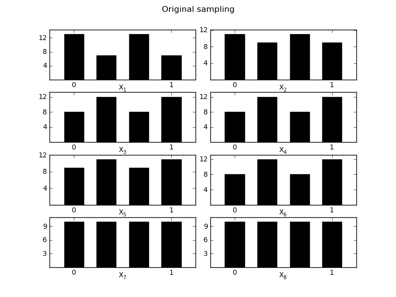
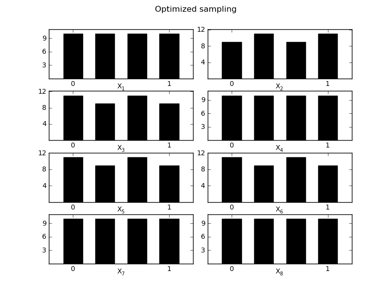
MorrisScreening.Optimized_diagnostic(width=0.1)

Evaluate the optimized trajects in their space distirbution, evaluation is done based on the [0-1] boundaries of the sampling

Returns quality measure and 2 figures to compare the optimized version

Parameters:

width : float

width of the bars in the plot (default 0.1)

Examples

>>> sm.Optimized_diagnostic()
The quality of the sampling strategy changed from 0.76 with the old
strategy to 0.88 for the optimized strategy

Output plots and exports

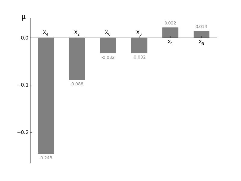
MorrisScreening.plotmu(width=0.5, addval=True, sortit=True, outputid=0, *args, **kwargs)

Plot a barchart of the given mu

mu is a measure for the first-order effect on the model output. However the use of mu can be tricky because if the model is non-monotonic negative elements can be in the parameter distribution and by taking the mean of the variance (= mu!) the netto effect is cancelled out! Should always be used together with plotsigma in order to see whether higher order effects are occuring, high sigma values with low mu values can be caused by non-monotonicity of functions. In order to check this use plotmustar and/or plotmustarsigma

Parameters:

width : float (0-1)

width of the bars in the barchart

addval : bool

if True, the morris mu values are added to the graph

sortit : bool

if True, larger values (in absolute value) are plotted closest to the y-axis

outputid : int

the output to use whe multiple are compared; starts with 0

*args, **kwargs : args

passed to the matplotlib.bar

Returns:

fig : matplotlib.figure.Figure object

figure containing the output

ax1 : axes.AxesSubplot object

the subplot

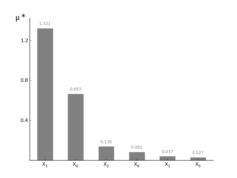
MorrisScreening.plotmustar(width=0.5, addval=True, sortit=True, outputid=0, *args, **kwargs)

Plot a barchart of the given mustar

mu* is a measure for the first-order effect on the model output. By taking the average of the absolute values of the parameter distribution, the absolute effect on the output can be calculated. This is very useful when you are working with non-monotonic functions. The drawback is that you lose information about the direction of influence (is this factor influencing the output in a positive or negative way?). For the direction of influence use plotmustar!

Parameters:

width : float (0-1)

width of the bars in the barchart

addval : bool

if True, the morris values are added to the graph

sortit : bool

if True, larger values (in absolute value) are plotted closest to the y-axis

outputid : int

the output to use whe multiple are compared; starts with 0

*args, **kwargs : args

passed to the matplotlib.bar; width is already used

Returns:

fig: matplotlib.figure.Figure object

figure containing the output

ax1: axes.AxesSubplot object

the subplot

MorrisScreening.plotsigma(width=0.5, addval=True, sortit=True, outputid=0, *args, **kwargs)

Plot a barchart of the given sigma

sigma is a measure for the higher order effects (e.g. curvatures and interactions). High sigma values typically occurs when for example parameters are correlated, the model is non linear,... The sum of all these effects is sigma. For linear models without any correlation sigma should be approximately zero.

Parameters:

width : float (0-1)

width of the bars in the barchart

addval : bool

if True, the morris values are added to the graph

sortit : bool

if True, larger values (in absolute value) are plotted closest to the y-axis

outputid : int

the output to use whe multiple are compared; starts with 0

*args, **kwargs : args

passed to the matplotlib.bar

Returns:

fig : matplotlib.figure.Figure object

figure containing the output

ax1 : axes.AxesSubplot object

the subplot

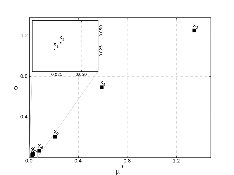
MorrisScreening.plotmustarsigma(outputid=0, zoomperc=0.05, loc=2)

Plot the mu* vs sigma chart to interpret the combined effect of both.

Parameters:

zoomperc : float (0-1)

the percentage of the output range to show in the zoomplot, if ‘none’, no zoom plot is added

loc : int

matplotlib.pyplot.legend: location code (0-10)

outputid : int

the output to use whe multiple are compared; starts with 0

Returns:

fig : matplotlib.figure.Figure object

figure containing the output

ax1 : axes.AxesSubplot object

the subplot

txtobjects : list of textobjects

enbales the ad hoc replacement of labels when overlapping

Notes

Visualization as proposed by [M2]

MorrisScreening.latexresults(outputid=0, name='Morristable.tex')

Print Results in a “deluxetable” Latex

Parameters:

outputid : int

teh output to use when evaluation for multiple outputs are calculated

name : str.tex

output file name; use .tex extension in the name

\begin{table}{lccc}
\tablewidth{0pc}
\tablecolumns{4}
\caption{Morris evaluation criteria\label{tab:morris1tot}}
\tablehead{
  & $\mu$ & $\mu^*$ & $\sigma$  }
\startdata
$X_1$ & 0.019 & 0.053 & 0.062\\
$X_2$ & -0.014 & 0.28 & 0.37\\
$X_3$ & 0.35 & 1.8 & 2.2\\
$X_4$ & 0.58 & 0.77 & 0.66\\
$X_5$ & -0.0091 & 0.029 & 0.035\\
$X_6$ & 0.023 & 0.088 & 0.11\\
\enddata
\end{table}

MorrisScreening.txtresults(outputid=0, name='Morrisresults.txt')

Results in txt file to load in eg excel

Parameters:

outputid : int

the output to use when evaluation for multiple outputs are calculated

name : str.txt

output file name; use .txt extension in the name

Par      mu      mustar          sigma
$X_1$    0.01923737       0.05295802      0.06235872
$X_2$    -0.01423402      0.27864841      0.36502709
$X_3$    0.35127671       1.79863549      2.19419533
$X_4$    0.57758340       0.76929478      0.66397173
$X_5$    -0.00912314      0.02933937      0.03503700
$X_6$    0.02319802       0.08834758      0.10503778

Standardized Regression Coefficients (SRC) method

Main SRC methods

class pystran.SRCSensitivity(parsin, ModelType='external')

The regression sensitivity analysis: MC based sampling in combination with a SRC calculation; the rank based approach (less dependent on linearity) is also included in the SRC calculation and is called SRRC

The model is proximated by a linear model of the same parameterspace and the influences of the parameters on the model output is evaluated.

Parameters:

parsin : list

Either a list of (min,max,’name’) values, [(min,max,’name’),(min,max,’name’),...(min,max,’name’)] or a list of ModPar instances

Notes

Rank transformation:

Rank transformation of the data can be used to transform a nonlinear but monotonic relationship to a linear relationship. When using rank transformation the data is replaced with their corresponding ranks. Ranks are defined by assigning 1 to the smallest value, 2 to the second smallest and so-on, until the largest value has been assigned the rank N.

Examples

>>> ai=np.array([10,20,15,1,2,7])
>>> Xi = [(8.0,9.0,r'$X_1$'),(7.0,10.0,r'$X_2$'),(6.0,11.0,r'$X_3$'),
>>>       (5.0,12.0,r'$X_4$'), (4.0,13.0,r'$X_5$'),(3.0,4.,r'$X_6$')]      
>>> #prepare method
>>> reg=SRCSensitivity(Xi)
>>> #prepare parameter samples
>>> reg.PrepareSample(1000)  
>>> #run model and get outputs for all MC samples
>>> output = np.zeros((reg.parset2run.shape[0],1))
>>> for i in range(reg.parset2run.shape[0]):
>>>     output[i,:] = simplelinear(ai,reg.parset2run[i,:])
>>> #Calc SRC without using rank-based approach
>>> reg.Calc_SRC(output, rankbased=False)
>>> #check if the sum of the squared values approaches 1
>>> print reg.sumcheck
>>> [ 1.00555193]
>>> reg.plot_tornado(outputid = 0, ec='grey',fc='grey')

Attributes

_ndim

( intx) number of factors examined. In case the groups are chosen the number of factors is stores in NumFact and sizea becomes the number of created groups, (k)

Calc_SRC(output, rankbased=False)

SRC sensitivity calculation for multiple outputs

Check is done on the Rsq value (higher than 0.7?) and the sum of SRC’s for the usefulness of the method.

Parameters:

output : Nxm ndarray

array with the model outputs (N MC simulations and m different outputs)

rankbased : boolean

if True, SRC values are transformed into SRRC values; using ranks instead of values itself

Notes

Least squares Estimation theory, eg. http://www.stat.math.ethz.ch/~geer/bsa199_o.pdf

Attributes

SRC	(ndimxnoutputs narray) Standardized Regression Coefficients
cova :	variance-Covariance matrix
core :	correlation matrix
sumcheck	(noutput narray) chek for linearity by summing the SRC values

PrepareSample(nbaseruns, samplemethod='Sobol', seedin=1)

Sampling of the parameter space. No specific sampling preprocessing procedure is needed, only a general Monte Carlo sampling of the parameter space is expected. To improve the sampling procedure, Latin Hypercube or Sobol pseudo-random sampling can be preferred. The latter is used in the pySTAN framework, but using the ModPar class individually enables Latin Hypercube and random sampling.

Currently only uniform distributions are supported by the framework, but the Modpar class enables other dsitributions to sample the parameter space and bypassing the sampling here.

Parameters:

nbaseruns : int

number of samples to take for the analysis; highly dependent from the total number of input factors. range of 10000s is minimum.

samplemethod : ‘sobol’ or ‘lh’

sampling method to use for the sampling

seedin : int

seed to start the Sobol sampling from. This enables to increase the sampling later on, by starting from the previous seedout.

Returns:

seed_out : int

the last seed, useful for later use

parset2run : ndarray

parameters to run the model (nbaseruns x ndim)

Notes

• Do the Sobol sampling always for the entire parameter space at the

same time, for LH this doesn’t matter! - Never extend the sampling size with using the same seed, since this generates duplicates of the samples!

Quick analysis of the scatter plots of the ouput versus the parameter values

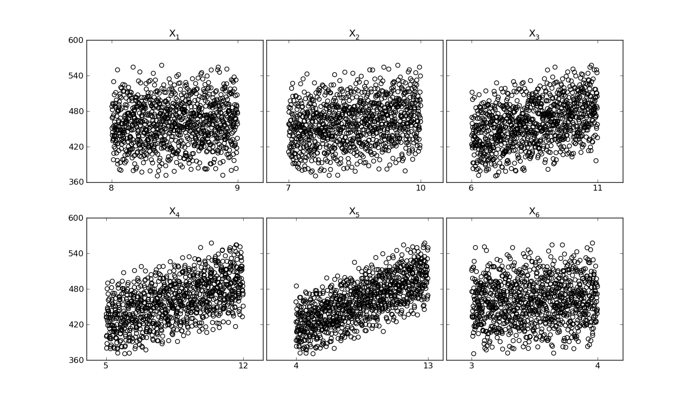
SRCSensitivity.quickscatter(output)

Quick link to the general scatter function, by passing to the general scattercheck plot of the sensitivity base-class

Parameters:

output: ndimx1 array

array with the output for one output of the model; this can be an Objective function or an other model statistic

Notes

Used to check linearity of the input/output relation in order to evaluate the usefulness of the SRC-regression based technique

Examples

>>> reg.quickscatter(output)

Output image:

Output plots and exports

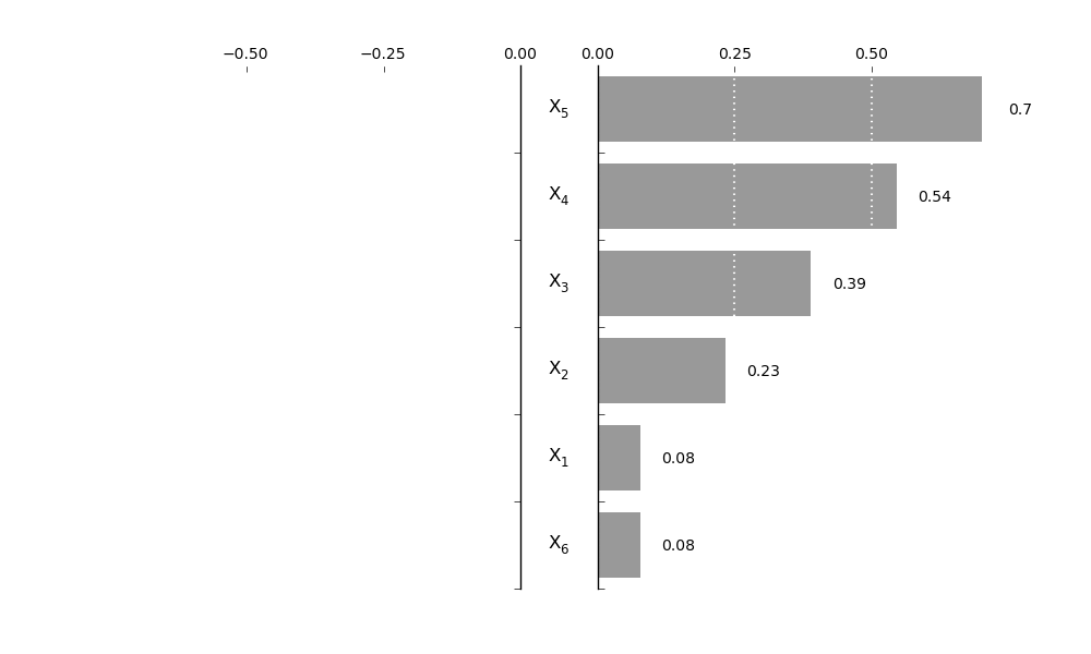
SRCSensitivity.plot_tornado(outputid=0, SRC=True, *args, **kwargs)

Make a Tornadplot of the parameter influence on the output; SRC must be calculated first before plotting

Parameters:

outputid : int

output for which the tornado plot is made, starting from 0

SRC : boolean

SRC true means that SRC values are used, otherwise the SRRC (ranked!) is used

*args, **kwargs :

arguments passed to the TornadoSensPlot function of the plotfunctions_rev data

Notes

The parameters for the tornadosensplot are:

gridbins: int, number of gridlines midwidth: float, width between the two axis, adapt to parameter names setequal: boolean, if True, axis are equal lengths plotnumb: boolean, if True, sensitiviteis are plotted parfontsize: int, font size of the parameter names bandwidth: width of the band

Examples

>>> reg.plot_tornado(outputid = 0,gridbins=3, midwidth=0.2, 
                     setequal=True, plotnumb=True, parfontsize=12, 
                     bandwidth=0.75)

Output image:

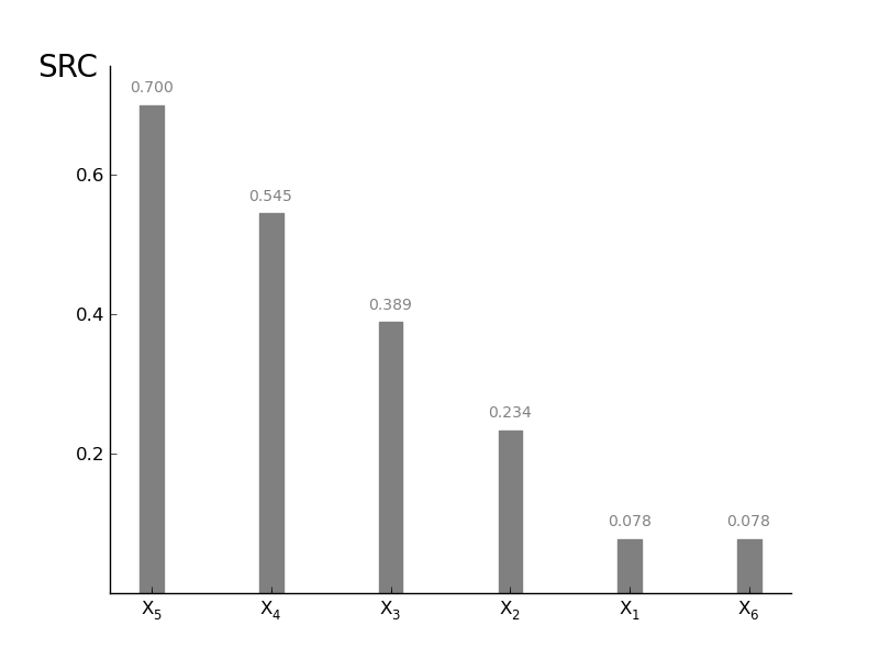
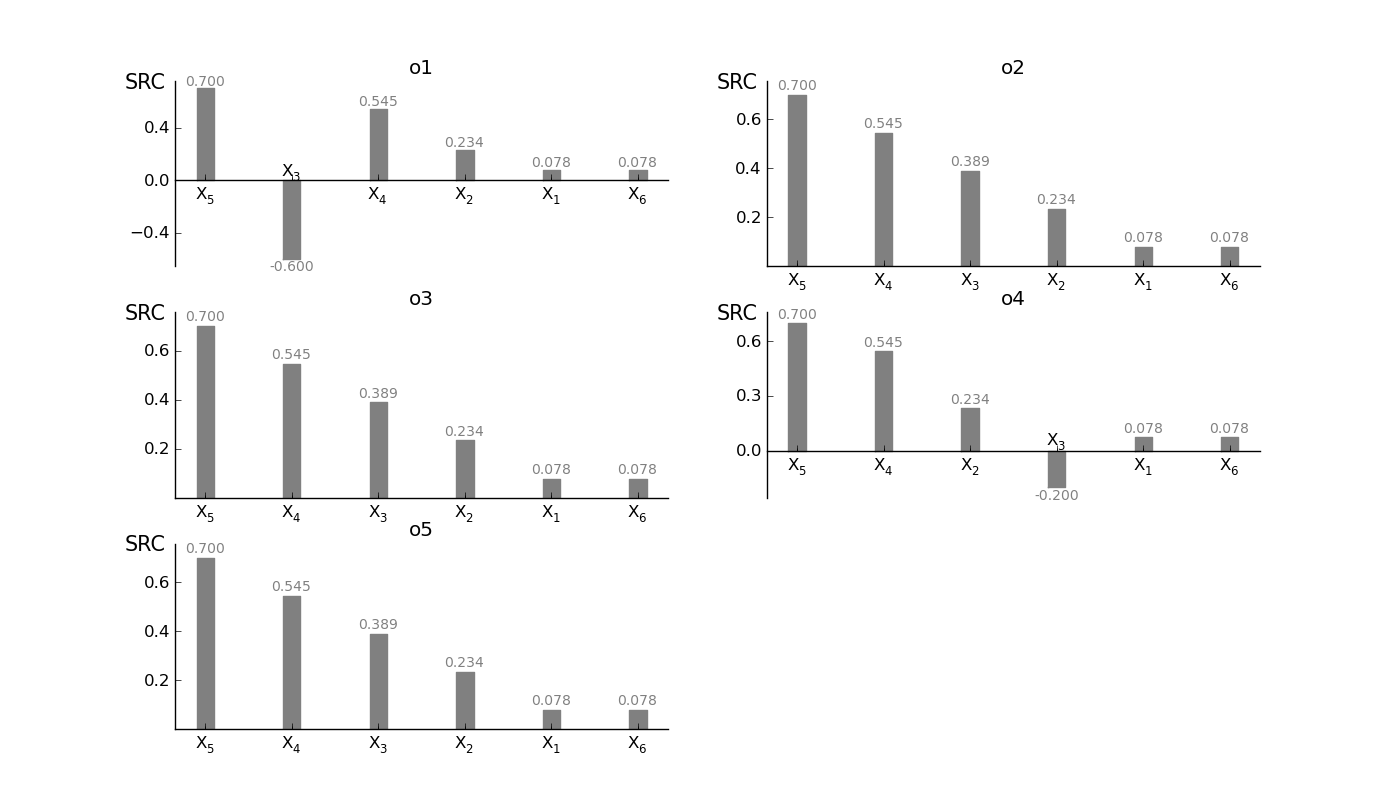
SRCSensitivity.plot_SRC(width=0.2, addval=True, sortit=True, outputid='all', ncols=3, outputnames=[], *args, **kwargs)

Plot a barchart of the SRC values; actually a Tornadoplot in the horizontal direction. More in the style of the other methods.

TODO: make for subset of outputs, also in other methods; currently all or 1

Parameters:

width : float (0-1)

width of the bars in the barchart

addval : bool

if True, the sensitivity values are added to the graph

sortit : bool

if True, larger values (in absolute value) are plotted closest to the y-axis

outputid : int or all

the output to use whe multiple are compared; starts with 0 if all, the different outputs are plotted in subplots

ncols : int

number of columns to put the subplots in

outputnames : list of strings

[] to plot no outputnames, otherwise list of strings equal to the number of outputs

*args, **kwargs : args

passed to the matplotlib.bar

Returns:

fig : matplotlib.figure.Figure object

figure containing the output

ax1 : axes.AxesSubplot object

the subplot

Examples

>>> #plot single SRC
>>> reg.plot_SRC(outputid=0, width=0.3, sortit = True, 
                 ec='grey',fc='grey')
>>> #plot single SRC (assume 4 outputs)      
>>> reg.plot_SRC(outputid = 'all' , ncols = 2, 
                  outputnames=['o1','o2','o3','o4'], ec='grey', fc='grey')

Output image if a single output is selected:

Output image if a all outputs are selected:

SRCSensitivity.latexresults(outputnames, rank=False, name='SRCtable.tex')

Print results SRC values or ranks in a “deluxetable” Latex

Parameters:

outputnames : list of strings

The names of the outputs in the colomns

rank : boolean

if rank is True, rankings or plotted in tabel instead of the SRC values

name : str.tex

output file name; use .tex extension in the name

\begin{table}{lccccc}
\tablewidth{0pc}
\tablecolumns{6}
\caption{Global SRC parameter ranking\label{tab:SRCresult}}
\tablehead{
 & o1 & o2 & o3 & o4 & o5  }
\startdata
$X_1$ & 5 & 5 & 5 & 5 & 5\\
$X_2$ & 4 & 4 & 4 & 4 & 4\\
$X_3$ & 3 & 3 & 3 & 3 & 3\\
$X_4$ & 2 & 2 & 2 & 2 & 2\\
$X_5$ & 1 & 1 & 1 & 1 & 1\\
$X_6$ & 6 & 6 & 6 & 6 & 6\\
\enddata
\end{table}

SRCSensitivity.txtresults(outputnames, rank=False, name='SRCresults.txt')

Results rankmatrix in txt file to load in eg excel

Parameters:

outputnames : list of strings

The names of the outputs in the colomns

rank : boolean

if rank is True, rankings or plotted in tabel instead of the SRC values

name : str.txt

output file name; use .txt extension in the name

Par      o1      o2      o3      o4      o5
$X_1$    0.0778505546741         0.0778505546741         0.0778505546741         0.0778505546741         0.0778505546741
$X_2$    0.233670804823  0.233670804823  0.233670804823  0.233670804823  0.233670804823
$X_3$    -0.6    0.389115599046  0.389115599046  0.389115599046  0.389115599046
$X_4$    0.544743494911  0.544743494911  0.544743494911  0.544743494911  0.544743494911
$X_5$    0.700482475678  0.700482475678  0.700482475678  0.700482475678  0.700482475678
$X_6$    0.0778270555871         0.0778270555871         0.0778270555871         0.0778270555871         0.0778270555871

Sobol Variance based method

Main Sobol variance methods

class pystran.SobolVariance(parsin, ModelType='pyFUSE')

Sobol Sensitivity Analysis Variance Based

Parameters:

ParsIn : list

either a list of (min,max,’name’) values, [(min,max,’name’),(min,max,’name’),...(min,max,’name’)] or a list of ModPar instances

ModelType : pyFUSE | PCRaster | external

Give the type of model working with

Notes

Calculates first and total order, and second order Total Sensitivity, according to [S1] , higher order terms and bootstrapping is not (yet) included

References

[S1]	(1, 2, 3, 4) Saltelli, A., P. Annoni, I. Azzini, F. Campolongo, M. Ratto, S. Tarantola,(2010) Variance based sensitivity analysis of model output. Design and estimator for the total sensitivity index, Computer Physics Communications, 181, 259–270

[S2]	(1, 2) Saltelli, Andrea, Marco Ratto, Terry Andres, Francesca Campolongo, Jessica Cariboni, Debora Gatelli, Michaela Saisana, and Stefano Tarantola. Global Sensitivity Analysis, The Primer. John Wiley & Sons Ltd, 2008.

Examples

>>> ai=[0, 1, 4.5, 9, 99, 99, 99, 99]
>>> alphai = 0.5 * np.ones(len(ai))
>>> Xi = [(0.0,1.0,'par1'),(0.0,1.0,'par2'),(0.0,1.0,'par3'),(0.0,1.0,'par4'),
      (0.0,1.0,'par5'),(0.0,1.0,'par6'),(0.0,1.0,'par7'),(0.0,1.0,'par8'),]
>>> di=np.random.random(8)
>>> #set up sensitivity analysis
>>> sens2 = SobolVariance(Xi, ModelType = 'testmodel')
>>> #Sampling strategy
>>> sens2.SobolVariancePre(1500)
>>> #Run model + evaluate the output
>>> sens2.runTestModel('analgfunc', [ai, alphai, di]) #here normally other model
>>> #results in txt file 
>>> sens2.txtresults(name='SobolTestOut.txt')
>>> #results in tex-table 
>>> sens2.latexresults(name='SobolTestOut.tex')
>>> #Plots
>>> sens2.plotSi(ec='grey',fc='grey')
>>> sens2.plotSTi(ec='grey',fc='grey')
>>> sens2.plotSTij()
>>> Si_evol, STi_evol = sens2.sens_evolution(color='k')    

Attributes

parset2run

(ndarray) every row is a parameter set to run the model for. All sensitivity methods have this attribute to interact with base-class running

SobolVariancePost(output, repl=1, adaptedbaserun=None, forevol=False)

Calculate first and total indices based on model output and sampled values

the sensmatrices for replica, have repititions in the rows, columns are the factors

only output => make multiple outputs (todo!!), by using the return, different outputs can be tested...

Parameters:

output : ndarray

Nx1 matrix with the model outputs

repl : int

number of replicates used

adaptedbaserun : int

number of baseruns to base calculations on

forevol : boolean

True if used for evaluating the evolution

Notes

The calculation methods follows as the directions given in [S1]

SobolVariancePre(nbaseruns, seed=1, repl=1, conditional=None)

Set up the sampling procedure of N*(k+2) samples

Parameters:

nbaseruns : int

number of samples for the basic analysis, total number of model runs is Nmc(k+2), with k the number of factors

seed : int

to set the seed point for the sobol sampling; enables to enlarge a current sample

repl : int

Replicates the entire sampling procedure. Can be usefull to test if the current sampling size is large enough to get convergence in the sensitivity results (bootstrapping is currently not included)

Notes

Following the Global sensitivity analysis, [S2], but updated for [S1] for more optimal convergence of the sensitivity indices

Sobolsampling(nbaseruns, seedin=1)

Performs Sobol sampling procedure, given a set of ModPar instances, or by a set of (min,max) values in a list.

This function is mainly used as help function, but can be used to perform Sobol sampling for other purposes

Todo: improve seed handling, cfr. bioinspyred package

Parameters:

nbaseruns : int

number of runs to do

seed : int

to et the seed point for the sobol sampling

Notes

DO SOBOL SAMPLING ALWAYS FOR ALL PARAMETERS AT THE SAME TIME!

Duplicates the entire parameter set to be able to divide in A and B matric

Examples

>>> p1 = ModPar('tp1',2.0,4.0,3.0,'randomUniform')    
>>> p2 = ModPar('tp2',1.0,5.0,4.0,'randomUniform')
>>> p3 = ModPar('tp3',0.0,1.0,0.1,'randomUniform')
>>> sobanal1 = SobolVariance([p1,p2,p3])
>>> sobanal2 = SobolVariance([(2.0,4.0,'tp1'),(1.0,5.0,'tp2'),(0.0,1.0,'tp3')])
>>> pars1 = sobanal.Sobolsampling(100,seed=1)
>>> pars2 = sobanal.Sobolsampling(100,seed=1)

runTestModel(model, inputsmod, repl=1)

Run a testmodel

Use a testmodel to get familiar with the method and try things out. The implemented methods are * G Sobol function: testfunction with analytical solution * gstarfunction: testfunction with analytical solution, extended version of the G sobol function

Parameters:

model : string

name fo the testmodel

inputsmod : list

list with all the inputs of the model, except of the sampled stuff

repl : int

Notes

More information on both testfunctions can be found in:

• G Sobol function [S2]
• G* function [S1]

Check the convergence of the analysis

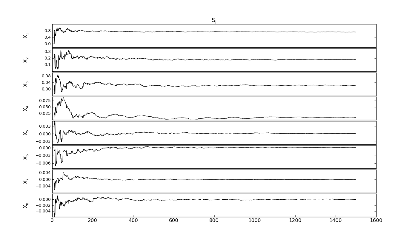
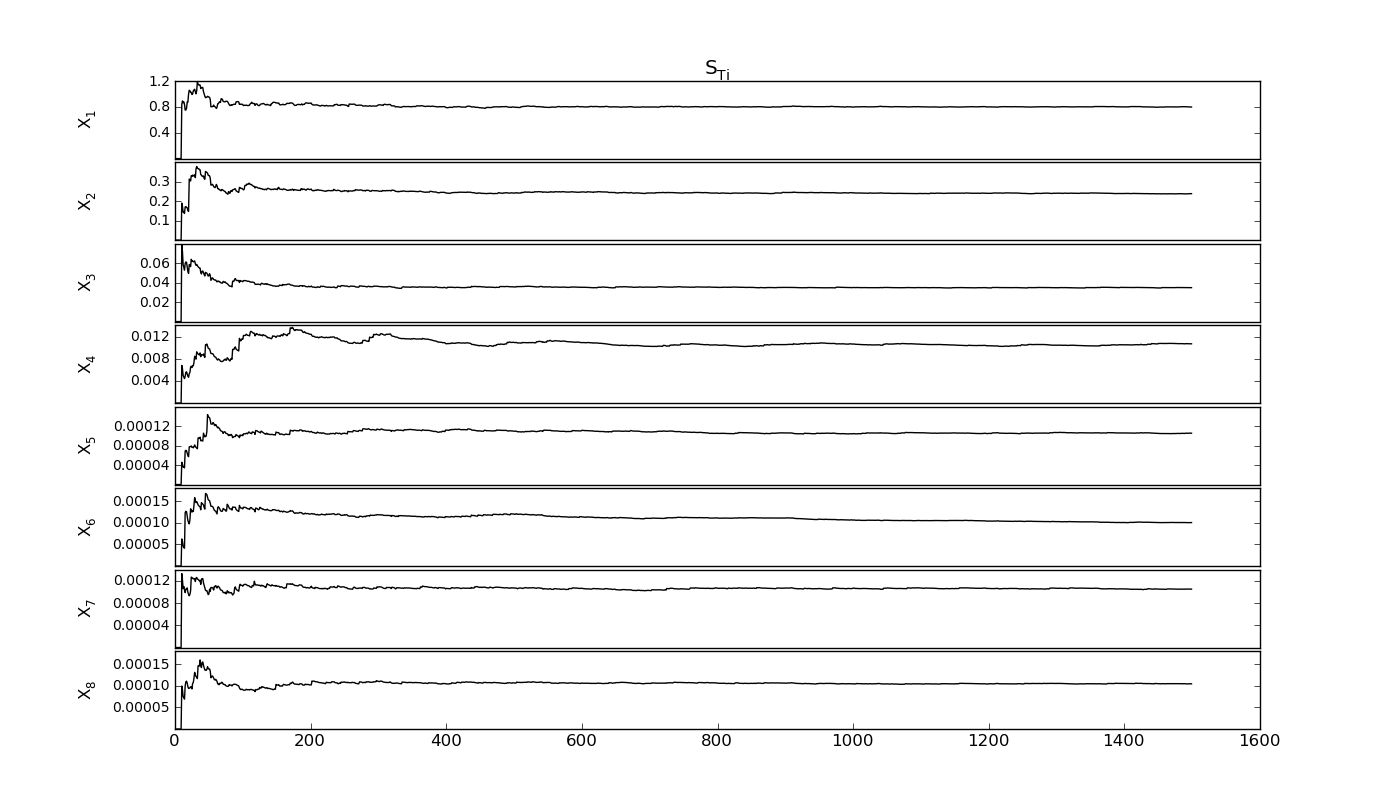
SobolVariance.sens_evolution(output=None, repl=1, labell=-0.07, *args, **kwargs)

Check the convergence of the current sequence

Parameters:

output : optional

if True; this output is used, elsewhere the generated output

repl : int

must be 1 to work

labell : float

aligns the ylabels

*args, **kwargs : args

passed to the matplotlib.plot function

Returns:

Si_evol : ndarray

Si of the factors in number of nbaseruns

STi_evol : ndarray

STi of the factors in number of nbaseruns

Output plots and exports

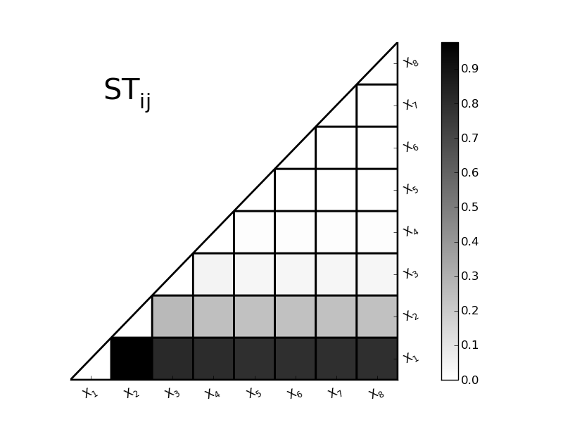
SobolVariance.plotSTij(linewidth=2.0)

Plot the STij interactive terms

Parameters:

linewidth : float

width of the black lines of the grid

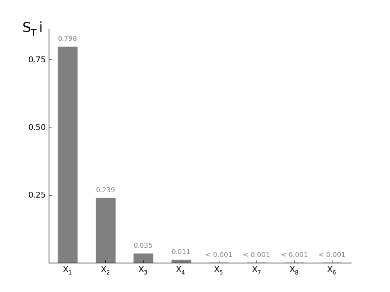
SobolVariance.plotSTi(width=0.5, addval=True, sortit=True, *args, **kwargs)

Plot a barchart of the given STi

Parameters:

width : float (0-1)

width of the bars in the barchart

addval : bool

if True, the morris mu values are added to the graph

sortit : bool

if True, larger values (in absolute value) are plotted closest to the y-axis

*args, **kwargs : args

passed to the matplotlib.bar

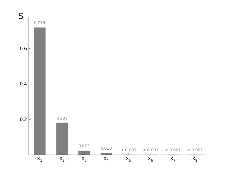
SobolVariance.plotSi(width=0.5, addval=True, sortit=True, *args, **kwargs)

Plot a barchart of the given Si

Parameters:

width : float (0-1)

width of the bars in the barchart

addval : bool

if True, the morris mu values are added to the graph

sortit : bool

if True, larger values (in absolute value) are plotted closest to the y-axis

*args, **kwargs : args

passed to the matplotlib.bar

SobolVariance.latexresults(name='Soboltable.tex')

Print Results in a “deluxetable” Latex

Parameters:

name : str.tex

output file name; use .tex extension in the name

\begin{table}{lcc}
\tablewidth{0pc}
\tablecolumns{3}
\caption{First order and Total sensitivity index\label{tab:sobol1tot}}
\tablehead{
  & $S_i$ & $S_{Ti}$  }
\startdata
par1 & 0.72 & 0.79\\
par2 & 0.18 & 0.24\\
par3 & 0.023 & 0.034\\
par4 & 0.0072 & 0.010\\
par5 & 0.000044 & 0.00011\\
par6 & 0.000068 & 0.00011\\
par7 & 0.000028 & 0.00010\\
par8 & 0.000049 & 0.00011\\
SUM & 0.93 & 1.1\\
\enddata
\end{table}

SobolVariance.txtresults(name='Sobolresults.txt')

Results in txt file to load in eg excel

Parameters:

name : str.txt

output file name; use .txt extension in the name

Par      Si      STi
par1     0.71602494       0.78797717
par2     0.17916175       0.24331297
par3     0.02346677       0.03437614
par4     0.00720168       0.01044238
par5     0.00004373       0.00010526
par6     0.00006803       0.00010556
par7     0.00002847       0.00010479
par8     0.00004918       0.00010522
SUM      0.92604455       1.07652948

Latin-Hypercube OAT method

Main GLobal OAT methods

class pystran.GlobalOATSensitivity(parsin, ModelType='external')

A merged apporach of sensitivity analysis; also extended version of the LH-OAT approach

Parameters:

parsin : list

either a list of (min,max,’name’) values, [(min,max,’name’),(min,max,’name’),...(min,max,’name’)] or a list of ModPar instances

Notes

Original method described in [OAT1], but here generalised in the framework, by adding different measures of sensitivity making the sampling method adjustable (lh or Sobol pseudosampling) and adding the choice of numerical approach to derive the derivative.

References

[OAT1]

(1, 2) van Griensven, Ann, T. Meixner, S. Grunwald, T. Bishop, M. Diluzio, and R. Srinivasan. ‘A Global Sensitivity Analysis Tool for the Parameters of Multi-variable Catchment Models’ 324 (2006): 10–23.

[OAT2]

(1, 2) Pauw, Dirk D E, D E Leenheer Decaan, and V A N Langenhove Promotor. OPTIMAL EXPERIMENTAL DESIGN FOR CALIBRATION OF BIOPROCESS MODELS : A VALIDATED SOFTWARE TOOLBOX OPTIMAAL EXPERIMENTEEL ONTWERP VOOR KALIBRERING VAN BIOPROCESMODELLEN : EEN GEVALIDEERDE SOFTWARE TOOLBOX BIOPROCESS MODELS : A VALIDATED SOFTWARE TOOLBOX, 2005.

Examples

>>> #EXAMPLE WITH ANALG-FUNCTION
>>> #variables and parameters
>>> ai=np.array([78, 12, 0.5, 2, 97, 33])
>>> Xi = [(0.0,1.0,r'$X_1$'),(0.0,1.0,r'$X_2$'),(0.0,1.0,r'$X_3$'),
          (0.0,1.0,r'$X_4$'), (0.0,1.0,r'$X_5$'),(0.,1,r'$X_6$')]    
>>> #prepare model class
>>> goat=GlobalOATSensitivity(Xi)
>>> #prepare the parameter sample
>>> goat.PrepareSample(100,0.01, 
                       samplemethod='lh', 
                       numerical_approach='central')
>>> #calculate model outputs                   
>>> output = np.zeros((goat.parset2run.shape[0],1))
>>> for i in range(goat.parset2run.shape[0]):
        output[i,:] = analgfunc(ai,goat.parset2run[i,:])
>>> #evaluate sensitivitu
>>> goat.Calc_sensitivity(output)
>>> #transform sensitivity into ranking
>>> goat.Get_ranking() 
>>> #plot the partial effect based sensitivity
>>> goat.plotsens(indice='PE', ec='grey',fc='grey')
>>> #plot the rankmatrix
>>> goat.plot_rankmatrix(outputnames)              

Attributes

_ndim

( intx) number of factors examined. In case the groups are chosen the number of factors is stores in NumFact and sizea becomes the number of created groups, (k)

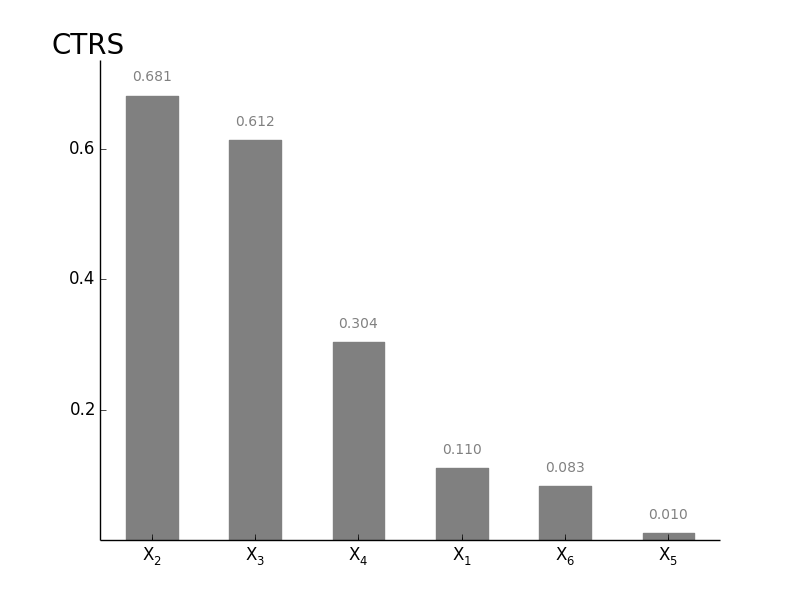
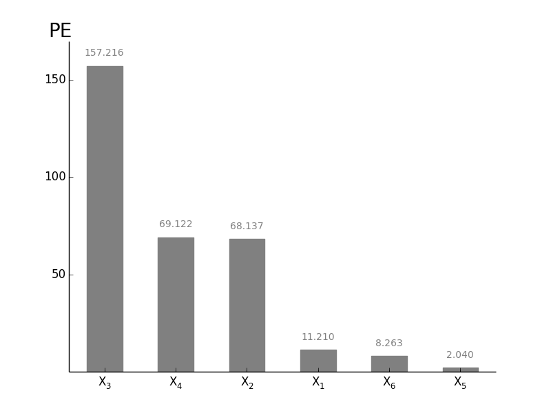
Calc_sensitivity(output)

Calculate the Central or Single Absolute Sensitvity (CAS), the Central or Single Total Sensitivity (CTRS) and the Partial Effect (PE) of the different outputs given. These outputs can be either a set of model objective functions or a timerserie output

Parameters:

output: Nxndim array

array with the outputs for the different outputs of the model; this can be an Objective function, or a timeserie of the model output

Notes

PE is described in [OAT1], the other two are just global extensions of the numercial approach to get local sensitivity results, see [OAT2].

Attributes

CAS_SENS:	Central/Single Absolute Sensitivity
CTRS_SENS:	Central/Single Total Sensitivity
PE_SENS:	Partial effect (van Griensven)

PrepareSample(nbaseruns, perturbation_factor, samplemethod='Sobol', numerical_approach='central', seedin=1)

Sampling of the parameter space. No specific sampling preprocessing procedure is needed, only a general Monte Carlo sampling of the parameter space is expected. To improve the sampling procedure, Latin Hypercube or Sobol pseudo-random sampling can be preferred. The latter is used in the pySTAN framework, but using the ModPar class individually enables Latin Hypercube and random sampling.

Currently only uniform distributions are supported by the framework, but the Modpar class enables other dsitributions to sample the parameter space and bypassing the sampling here.

Parameters:

nbaseruns : int

number of samples to take for the analysis; highly dependent from the total number of input factors. range of 10000s is minimum.

perturbation_factor : float or list

if only one number, all parameters get the same perturbation factor otherwise, _ndim elements in list

samplemethod : ‘sobol’ or ‘lh’

sampling method to use for the sampling

numerical_approach : ‘central’ or ‘single’

central approach needs n(2*k) runs, singel only n(k+1) runs; OAT calcluation depends on this.

seedin : int

seed to start the Sobol sampling from. This enables to increase the sampling later on, by starting from the previous seedout.

Returns:

seed_out : int

the last seed, useful for later use

parset2run : ndarray

parameters to run the model (nbaseruns x ndim)

Notes

• Do the Sobol sampling always for the entire parameter space at the

same time, for LH this doesn’t matter * Never extend the sampling size with using the same seed, since this generates duplicates of the samples * More information about the central or single numerical choice is given in [OAT2].

Output plots and exports

GlobalOATSensitivity.Get_ranking(choose_output=False)

Only possible if Calc_sensitivity is already finished; every columns gets is one ranking and the overall_importance is calculated based on the lowest value of the other rankings (cfr. Griensven)

rankmatrix: defines the rank of the parameter self.rankdict: defines overall rank of the parameters with name

Parameters:

choose_output: integer

starting from 1 as the first output

Notes

TODO make a dataframe of pandas as output: rows is par, cols is output

Attributes

rankdict (only when single output selected):	Dictionary giving the ranking of the parameter
rankmatrix:	Main output: gives for each parameter (rows) the ranking for the different outputs
overall_importance:	Returns the summarized importance of the parameter over the different outputs, by checking the minimal ranking of the parameters

GlobalOATSensitivity.plotsens(indice='PE', width=0.5, addval=True, sortit=True, outputid=0, *args, **kwargs)

Plot a barchart of either CAS, CTRS or PE based Senstivitity

Parameters:

indice: PE, CAS or CTRS

choose which indice you want to show

width : float (0-1)

width of the bars in the barchart

addval : bool

if True, the sensitivity values are added to the graph

sortit : bool

if True, larger values (in absolute value) are plotted closest to the y-axis

outputid : int

the output to use whe multiple are compared; starts with 0

*args, **kwargs : args

passed to the matplotlib.bar

Returns:

fig : matplotlib.figure.Figure object

figure containing the output

ax1 : axes.AxesSubplot object

the subplot

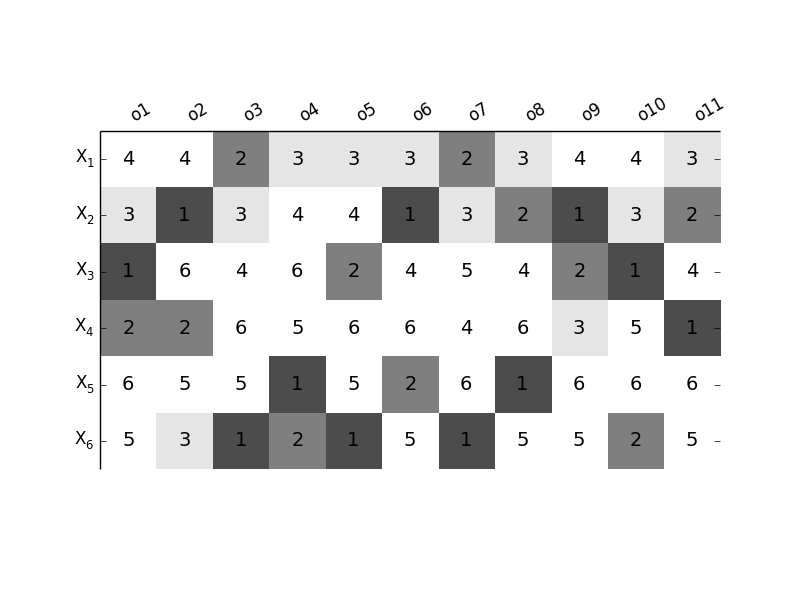
GlobalOATSensitivity.plot_rankmatrix(outputnames, fontsize=14)

Make an overview plot of the resulting ranking of the different parameters for the different outputs

Parameters:

outputnames : list of strings

The names of the outputs in the colomns

fontsize: int

size of the numbers of the ranking

GlobalOATSensitivity.latexresults(outputnames, name='GlobalOATtable.tex')

Print results rankmatrix in a “deluxetable” Latex

Parameters:

outputnames : list of strings

The names of the outputs in the colomns

name : str.tex

output file name; use .tex extension in the name

\begin{table}{lccccccccccc}
\tablewidth{0pc}
\tablecolumns{12}
\caption{Global OAT parameter ranking\label{tab:globaloatrank}}
\tablehead{
 & o1 & o2 & o3 & o4 & o5 & o6 & o7 & o8 & o9 & o10 & o11  }
\startdata
$X_1$ & 4 & 4 & 2 & 3 & 3 & 3 & 2 & 3 & 4 & 4 & 3\\
$X_2$ & 3 & 1 & 3 & 4 & 4 & 1 & 3 & 2 & 1 & 3 & 2\\
$X_3$ & 1 & 6 & 4 & 6 & 2 & 4 & 5 & 4 & 2 & 1 & 4\\
$X_4$ & 2 & 2 & 6 & 5 & 6 & 6 & 4 & 6 & 3 & 5 & 1\\
$X_5$ & 6 & 5 & 5 & 1 & 5 & 2 & 6 & 1 & 6 & 6 & 6\\
$X_6$ & 5 & 3 & 1 & 2 & 1 & 5 & 1 & 5 & 5 & 2 & 5\\
\enddata
\end{table}

GlobalOATSensitivity.txtresults(outputnames, name='GlobalOATresults.txt')

Results rankmatrix in txt file to load in eg excel

Parameters:

outputnames : list of strings

The names of the outputs in the colomns

name : str.txt

output file name; use .txt extension in the name

Par      o1      o2      o3      o4      o5      o6      o7      o8      o9      o10     o11
$X_1$    4       4       2       3       3       3       2       3       4       4       3
$X_2$    3       1       3       4       4       1       3       2       1       3       2
$X_3$    1       6       4       6       2       4       5       4       2       1       4
$X_4$    2       2       6       5       6       6       4       6       3       5       1
$X_5$    6       5       5       1       5       2       6       1       6       6       6
$X_6$    5       3       1       2       1       5       1       5       5       2       5

Dynamic Identifiability Analysis (DYNIA)

added soon

Regional Sensitivity Analysis (RSA)

Extra info added soon

Main RSA methods

class pystran.RegionalSensitivity(parsin, ModelType='pyFUSE')

Regional Sensitivity Analysis (Monte Carlo Filtering).

Parameters:

ParsIn : list

either a list of (min,max,’name’) values, [(min,max,’name’),(min,max,’name’),...(min,max,’name’)] or a list of ModPar instances

ModelType : pyFUSE | PCRaster | external

Give the type of model working with

Notes

The method basically ranks/selects parameter sets based on a evaluation criterion and checks the marginal influence of the different parameters on this criterion. In literature, the method is known as Regional Sensitivity Analysis (RSA, [R1]), but also describe in [R2] and referred to as Monte Carlo Filtering. Intially introduced by [R1] with a split between behavioural and non-behavioural accombined with a Kolmogorov- smirnov rank test (necessary, but nof sufficient to determine insensitive), applied with ten-bins split of the behavioural by [R3] and a ten bins split of the entire parameter range by [R4].

The method is directly connected to the GLUE approach, using the behavioural simulation to define prediction limits of the model output. Therefore, this class is used as baseclass for the GLUE uncertainty.

References

[R1]	(1, 2) Hornberger, G.M., and R.C. Spear. An Approach to the Preliminary Analysis of Environmental Systems. Journal of Environmental Management 12 (1981): 7–18.

[R2]	Saltelli, Andrea, Marco Ratto, Terry Andres, Francesca Campolongo, Jessica Cariboni, Debora Gatelli, Michaela Saisana, and Stefano Tarantola. Global Sensitivity Analysis, The Primer. John Wiley & Sons Ltd, 2008.

[R3]	Freer, Jim, Keith Beven, and Bruno Ambroise. Bayesian Estimation of Uncertainty in Runoff Prediction and the Value of Data: An Application of the GLUE Approach. Water Resources Research 32, no. 7 (1996): 2161. http://www.agu.org/pubs/crossref/1996/95WR03723.shtml.

[R4]	Wagener, Thorsten, D. P. Boyle, M. J. Lees, H. S. Wheater, H. V. Gupta, and S. Sorooshian. A Framework for Development and Application of Hydrological Models. Hydrology and Earth System Sciences 5, no. 1 (2001): 13–26.

PrepareSample(nbaseruns, seedin=1)

Sampling of the parameter space. No specific sampling preprocessing procedure is needed, only a general Monte Carlo sampling of the parameter space is expected. To improve the sampling procedure, Latin Hypercube or Sobol pseudo-random sampling can be preferred. The latter is used in the pySTAN framework, but using the ModPar class individually enables Latin Hypercube and random sampling.

Currently only uniform distributions are supported by the framework, but the Modpar class enables other dsitributions to sample the parameter space and bypassing the sampling here.

Parameters:

nbaseruns : int

number of samples to take for the analysis; highly dependent from the total number of input factors. range of 10000s is minimum.

seedin : int

seed to start the Sobol sampling from. This enables to increase the sampling later on, by starting from the previous seedout.

Returns:

seed_out : int

the last seed, useful for later use

parset2run : ndarray

parameters to run the model (nbaseruns x ndim)

Notes

• Do the Sobol sampling always for the entire parameter space at the

same time, for LH this doesn’t matter * Never extend the sampling size with using the same seed, since this generates duplicates of the samples

checkprobs(arrtocheck)

select_behavioural(output, method='treshold', threshold=0.0, percBest=0.2, norm=True, mask=True)

Select bevahvioural parameter sets, based on output evaluation criterion used. w The algorithm makes only a ‘mask’ for further operation, in order to avoid memory overload by copying matrices

Parameters:

threshold :

output : ndarray

Nx1

Method can be ‘treshold’ based or ‘percentage’ based

All arrays must have same dimension in 0-direction (vertical); output-function only 1 column

InputPar is nxnpar; output is nx1; Output nxnTimesteps

this most be done for each structure independently

Output of OFfunctions/Likelihoods normalised or not (do it if different likelihoods have to be plotted together)

Generalised Likelihood Uncertainty Estimation (GLUE)

added soon